Snowflake Billing
Understanding Snowflaking billing and how to track this within the Kleene app
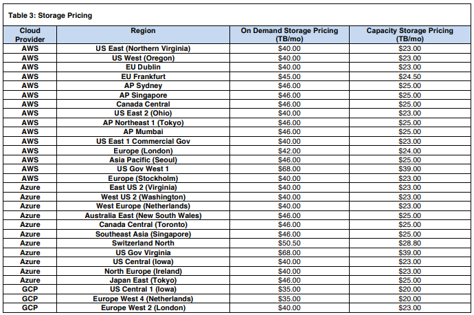
Snowflake credits are used to pay for the consumption of resources. The cost of a credit depends on the edition of Snowflake which the client has purchased.
There are three categories of Snowflake charges:
| Type of Cost | Comments |
|---|---|
| Data Storage | Calculated on the daily average amount of data stored in the system, charged per TB of storage |
| Compute Costs | These are generated by running extracts, by transforms and BI tools querying data in the warehouse |
| Cloud Services | Snowflake charges 4.4 credits per computer hour for Cloud Services, but only if the daily cost is more than 10% of the daily compute costs otherwise it is free. |
In practice, the Cloud Services cost rarely applies because the Compute Costs are high enough that the 10% threshold is not often exceeded.
The Storage costs effectively function as a flat charge, since few clients go over 1 TB of storage.

This means that the Compute Costs are the only type of cost that can be managed downwards.
Warehouses in Snowflake
A virtual warehouse is a set of compute resources that enable customers to execute queries, load data etc. Credits are used to pay for the processing time used by each virtual warehouse. The amount of credits charged per hour depends on the size of the warehouse - larger warehouses are significantly more expensive.

However a smaller warehouse runs more slowly. As queries are submitted to a warehouse, the warehouse allocates resources to each query. If sufficient resources are not available to execute all the queries, Snowflake queues the additional queries until the necessary resources become available. A larger warehouse makes more compute resources available, with less need for queuing.
A larger warehouse can therefore be cost effective when large amounts of data are being processed because although the cost per hour is higher, the time taken to process the data is shorter.
Most Kleene clients start on XS or S warehouses.
Multi-cluster warehouses
With multi-cluster warehouses, Snowflake allocates additional warehouses to make a larger pool of compute resources available. This can be done dynamically by Snowflake, which starts and stops different sizes of warehouse in response to the current load. This is useful where the load fluctuates unpredictably by large amounts.
How does warehouse billing work?
Snowflake only charges when the warehouse is actually running.
Auto-suspend: enabling auto-suspend means that the warehouse automatically suspends when there is no activity for a specified period of time. Snowflake recommends this period is set to a low value (e.g. 5 minutes or less) to avoid consuming credits when it is not running.
When the warehouse is suspended there are no charges - the exception is that the first minute is always charged in full even if the warehouse runs for less than a minute:
- The minimum billing charge is 1 minute, so there is no benefit to stopping a warehouse before the first minute because the credits have already been billed
- After the first minute, charges are incurred per second
- If the warehouse shuts down and then restarts, then a full minutes worth of charges will be billed again, e.g. if a warehouse runs for 61 seconds, shuts down, and then restarts and runs for less than 60 seconds, it is billed for 121 seconds (60 + 1 + 60)
It is therefore costly to start and stop the warehouse unnecessarily.
Caching
When a warehouse runs it builds up a cache of data from queries are processed by the warehouse. This enables improved performance for subsequent queries if they are able to read from the cache instead of from the tables in the query. The size of the cache is determined by the compute resources in the warehouse (i.e. the larger the warehouse and, therefore, more compute resources in the warehouse), the larger the cache.
When a warehouse is suspended, the cache is lost and has to be built up again - sometimes the performance improvement from using the cached data can make it worth keeping warehouses running for longer.
Recommendations for reducing Snowflake costs
Given that starting and stopping warehouses is costly, when running extracts and transforms we should aim to keep them running continuously.
- Run all the extracts within the same hour. Scheduling queries at exactly the same time should be avoided where rate limits are an issue (e.g. with the Facebook API)
- Look at the logs to understand how long the extracts take to run and set the transforms to run immediately afterwards
- Remember that if the client is using BI tools to query Snowflake then this generates compute costs as well, so these queries should run directly after the transforms
- Use incremental loads if possible, and for large datasets run transforms only the incremental data
- Use UNION ALL in preference to UNION (if there are definitely no duplicates in the dataset)
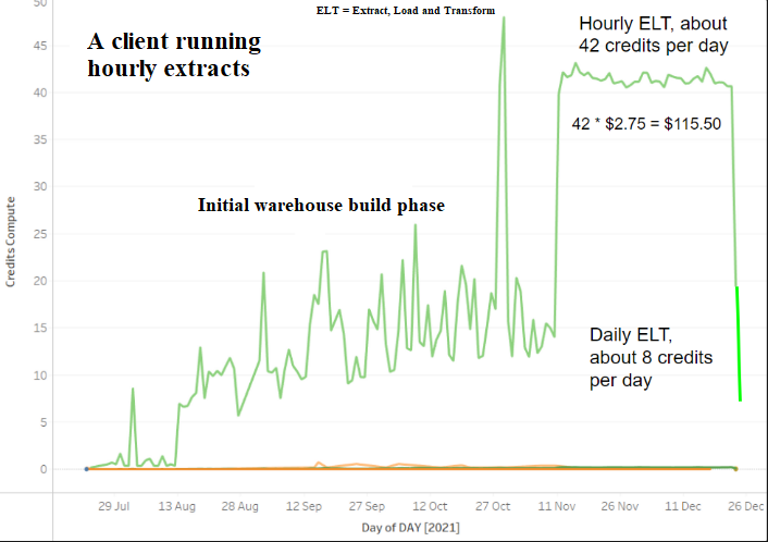
- Running hourly extracts is very expensive:

Measuring costs in Snowflake
The code to grant access to the SNOWFLAKE database is as follows:
grant imported privileges on database snowflake to role ELTThis query must be run from a user with a role that has ACCOUNTADMIN permissions. This is typically the user that set up the Snowflake account.
This database contains the ACCOUNT_USAGE schema and the METERING_HISTORY and METERING_DAILY_HISTORY views. This can be used to used to return the hourly credit usage for an account, METERING_DAILY_HISTORY gives the breakdown between Compute Costs and Cloud Services costs.
Consumption table: https://www.snowflake.com/legal-files/CreditConsumptionTable.pdf
Example SQL metering statement:
create schema if not exists utility;

CREATE OR REPLACE TABLE utility.snowflake_billing AS
select
      date_trunc(day, start_time)           as day
    , warehouse_name
    , sum(credits_used)                     as credits_total
    , sum(credits_used_compute)             as credits_compute
    , sum(credits_used_cloud_services)      as credits_cloud_services
from snowflake.account_usage.WAREHOUSE_METERING_HISTORY
group by 1,2
order by 1 desc
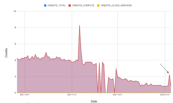
Example of charts produced by this data:

Updated 6 months ago
